Practical Strategies for Camera Exposure Management
Modern electronics are a wonderful thing. The matrix metering systems in today’s cameras are extremely sophisticated and will do a good job the majority of times. But that’s just it – not always. Leaving the camera on automatic is giving control to a machine for the most critical and creative aspects of your photography.
Digital camera metering systems work by taking multiple readings from the scene and then ‘averaging’ out the result. The camera then adjusts using sophisticated heuristics to counter the problem that average is not necessarily right.
There are two fundamental problems with leaving the camera on automatic or program modes. Firstly, there is a high possibility of getting things badly wrong and not being able to recover the file in post-processing – in short, blown highlights.
Secondly, the choices of ISO, aperture and shutter speed are actually crucial creative decisions. These settings adjust the depth of field and decide how the instant of time is rendered in the picture – from frozen action to blurred movement.
The automatic modes in cameras are a hangover from the film era – when the vast majority of people didn’t really understand or need to understand how exposure worked. Digital cameras introduced one feature that makes those modes mostly obsolete – the live-view histogram. I have made almost every digital exposure with my main cameras on manual mode for years now assisted by the live-view histogram and the purpose of this article is to explain how to always make the right exposure.
It’s also important to understand what we mean by ‘right’ exposure. It helps to recognise the distinction between the negative and the print – or in digital terms the raw file and the processed image (processed in raw editing software like Capture One or Lightroom). Ansel Adams said the negative is the score, the print is the performance. The goal of the negative (or raw file) is to capture the detail so that the vision for the print can be realised. Too little or too much light entering the camera can make producing the print difficult or even impossible.
So the goal is to take control of the exposure, shutter speed and aperture choices by using manual exposure modes. But how do you do this reliably? The answer is involved but essentially you follow similar strategies to those that were successful with film.
The principles of exposure
Highlight clipping
It’s worth starting from what you would do if you were metering a scene with a handheld light meter. I had to do this for a while with my IQ3 100. Digital sensors require the same strategy as film because they behave in essentially the same way as transparency film behaved in one important aspect – highlights can be clipped. Overexpose or blow the highlights and there is no way to recover the lost detail. Velvia transparency film used to blow detail over +1.7 stops above the metered reading. So to meter a scene for white water, snow or a wedding dress in the sun one had to meter the white/bright point and add 1.7 stops of exposure. Any more and detail in the white would be lost.
The same would apply for a digital sensor metered with a light meter, except the point of clipping is somewhere between 2 and 3 stops – it varies by camera and sensor. So generally to be safe we can add just over 2 stops of light from a metered highlight. For the IQ3 I aimed for placing the highlights at about +2.3 stops and always got great files.
Negative film is the same logic in reverse – the shadows clip (well, roll off so quickly that it amounts to the same thing) so one typically meters from the darkest point you want to have detail and reduces exposure by about 2 stops to place that point at the toe of the film.
This is where the histogram comes in for digital cameras. To expose for the highlights, use the live-view histogram in camera to place the highlight pixels close to the right-hand side of the graph without any clipping – i.e. no right-hand side spike and no flashing highlight pixels.
See this example from my Phase back on a technical camera. The lens is not connected to the back so it does not show the correct aperture but I used movements to adjust the plane of focus so that everything was sharp and set an aperture of f/11 on the Rodenstock 120mm lens with a shutter speed of 1/5th of a second. At ISO 100 this placed my highlights close to the edge of the sensor’s clipping point but with confidence that they have not clipped. Most pixels fall well within a range of 4–5 stops of light and I have no worries of losing any detail. No lost highlights and easily recovered shadows create a digital negative that is perfect for me to choose how to process and interpret my print.
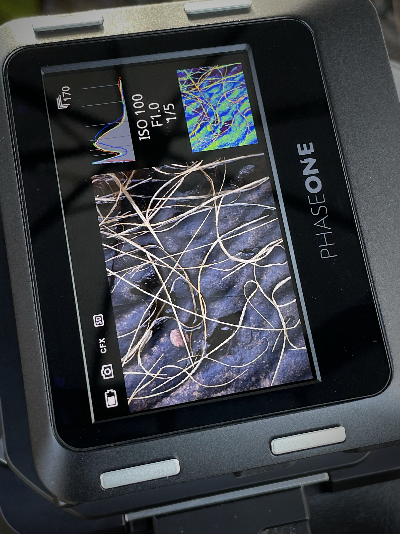
Crucially, digital cameras also have tools to check/review the histogram for an image already captured. One can confirm that it does not have clipped highlights and has a histogram distribution you were expecting – no spike at the right-hand side – so you can confirm that an image is exposed without problems and iterate if necessary. Doing this as a matter of course – in particular looking for the brightest spots – ensures that the exposure is captured well.
So the first takeaway should be to always expose for the important bright highlights – place them close to the clipping point but not actually risking any clipping.
Midtone and shadow quality
The second key concept is to make sure the midtones and shadows can be rendered with quality and accuracy in the final print.
Here again we come to one key difference between digital sensors and film. If you shoot in raw and capture the data hitting the sensor you have a significant latitude to move the exposure around – make the image brighter or darker – without causing the colour quality to collapse or the noise to increase.
Film had a toe – basically a non-linear transition to the film base with detail gradually disappearing. On transparency film it was 2–3 stops before detail was lost. And there was very little latitude to adjust anything once the exposure was made and the film developed. Typically midpoint exposure had to be accurate to within a third of a stop for well exposed transparencies. On negative film there could be as much as 10 or more stops of highlight detail to work with.
Digital sensors instead have a noise floor. The signal-to-noise ratio gradually decreases the further into the shadows one looks until the noise overwhelms the signal.
The latitude depends on the sensor – earlier sensors were limited to a couple of stops before noise and colour quality deteriorated but the latest BSI sensors can easily render 5–6 stops of detail recovered from the shadows more or less with impunity.
The practical consequence for most modern sensors is that in most low or medium contrast situations we can ignore the midtones and shadows. Just use the live-view histogram to expose for the highlights without risk of clipping and all is good.
But for transparency film it’s worth reviewing how to meter. Basically the handheld meter assumes what is being read is a midtone grey. So I would place dark greens on -1 (reduce exposure from the metered value by a stop), regular greens like grass on 0 or +0.3 and bright yellow on +1 (increase exposure by one stop from the metered spot).
This approach with a handheld meter will also get good results on digital sensors but is unnecessary if one places the highlights correctly using the live-view histogram.
High-contrast scenes
The scenario to worry about is what to do when the number of stops of light between the brightest point and the darkest point in the scene we want to render with detail is greater than the capacity of the sensor or film to handle well – retain detail, no noise, quality colour etc. This will happen frequently with landscape photography especially when photographing towards the sun or brightly lit clouds or when the sun is out and there is a range in the scene from sunlit white objects to deep shadows.
These situations can be identified based on experience or by reviewing the live-view histogram. If the highlights are placed correctly and there is a major spike in the extreme left of the histogram we may need to take action.
There are several main strategies:
Graduated ND filters – objects like bright skies can be darkened by adding a neutral density filter to the front of the lens. I still carry and use a 2-stop graduated ND filter for many high-contrast situations even on digital and of course this was the go-to strategy for balancing highlights, midpoints and shadows on transparency film.
Double exposure – the second strategy is to expose as close to the highlight clipping point as possible (without actually clipping) and make a first exposure followed immediately by a second image at +2. Most cameras can do this bracketing automatically. And then blend the two images in post-processing software (Capture One or Lightroom). My Phase back achieves this blend in camera without the post-processing step.
Push to the sensor’s true edge – I mentioned that Velvia had a +1.7 clipping barrier. That was empirically tested. Digital sensors have a similar clipping point and it is possible to maximise the dynamic range of the sensor by pushing it right to the edge. It will typically lie around +2.7 to +3. It’s important to understand that the histogram is actually based on a JPG conversion in most cameras not the actual raw data. The consequence is that the clipping point for the histogram or the highlight blinkies typically has a little latitude. If the JPG conversion applies a high-contrast curve, the histogram clips faster than the raw sensor does. It is possible to apply very low-contrast JPGs in camera (the Sony cameras can be set up this way) to get a more accurate clipping point. In the case of the Phase One IQ4 150 the camera uses raw data for the histogram so the clipping can be accurately assessed.
It is probably impractical today to use a handheld meter and learn the exact clipping point for your sensor but that would be the precise solution. The reality is that it’s much better to give yourself some contingency and deal with or live with the noise in post than risk clipping. The number of times that I actually messed up the highlights on transparency film was more than I would care to admit – at least in the early days. With digital the option to bracket up to the edge is of course available. So bracketing in 1/3-stop increments is a practical route.
Noise reduction – use post-processing software to reduce noise and improve the signal. It’s worth recognising that noise visible at 100% on a bright monitor is quite often invisible when a print is made.
Allow clipping – there are some situations where specular highlights and non-important highlights can be allowed to clip. In such situations I would still normally bracket and make another image with the highlights protected.
ETTR should be EFTH (‘Expose For The Highlights’)
There is one more nuance on digital that must be mentioned but then roundly ignored.
When base ISO is used, the sensor captures detail with more fidelity or levels of tonality the brighter the exposure. So a midtone captured at +2 to +2.5 will be captured with roughly 4–6× more levels than when it is exposed exactly on a midtone. This science combined with a simplified reading of the ‘expose for the highlights’ principles has led to the worst piece of advice ever given to beginners – you should always Expose to the Right (ETTR).
A midtone already carries more tonal information than any print can show so shifting the midtones by two further stops gains nothing useful. You are never going to see noise in a print of a midtone at base ISO, period.
And it has a catastrophic failure mode. Arbitrarily high exposure or exposure to the right risks highlight clipping.
ETTR should really be consigned to the dustbin of photographic misinformation alongside the ‘Rules of Composition’ and ‘I never use Photoshop to process my images because I want them to look how it actually was’. Think instead EFTH – Expose For The Highlights.
It is worth also adding one final nuance. A lot of recent sensors are dual gain. What this practically means is that there are two specific ISO levels where the optimum dynamic range is available. One can set the ISO at one of these two levels and then select the aperture and shutter speed as required. For example my Fuji GFX 100 II is optimal at base ISO (80) and at ISO 500. Dynamic range peaks at base and falls as ISO rises; at ~500 the sensor switches to its second, higher-gain readout, which cuts read noise and claws some dynamic range back. So on a tripod I would shoot at ISO 80 and handheld usually at ISO 500. Nothing is to be gained by setting the ISO outside these two settings (versus simply underexposing which will create the same effective raw data file) – i.e. underexposing by two stops at ISO 100 is the same as shooting at ISO 400. Each camera has different characteristics like this and it is helpful but not essential to understand your own camera.
Practical examples
Here are ten real world examples. If you can glance at these scenes and immediately know a) how you would expose for them with your camera and b) what to watch out for and what could go wrong then you are in good shape.
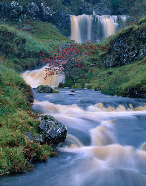
Example I was shot on transparency film – the whites in the river were spot metered and placed on +1.7. On digital the histogram highlights would be placed close to the right-hand side with no concern about midtone or shadow quality as the scene is low contrast. On negative film I would spot meter for the dark shadows in the side of the river and reduce exposure by just under two stops.
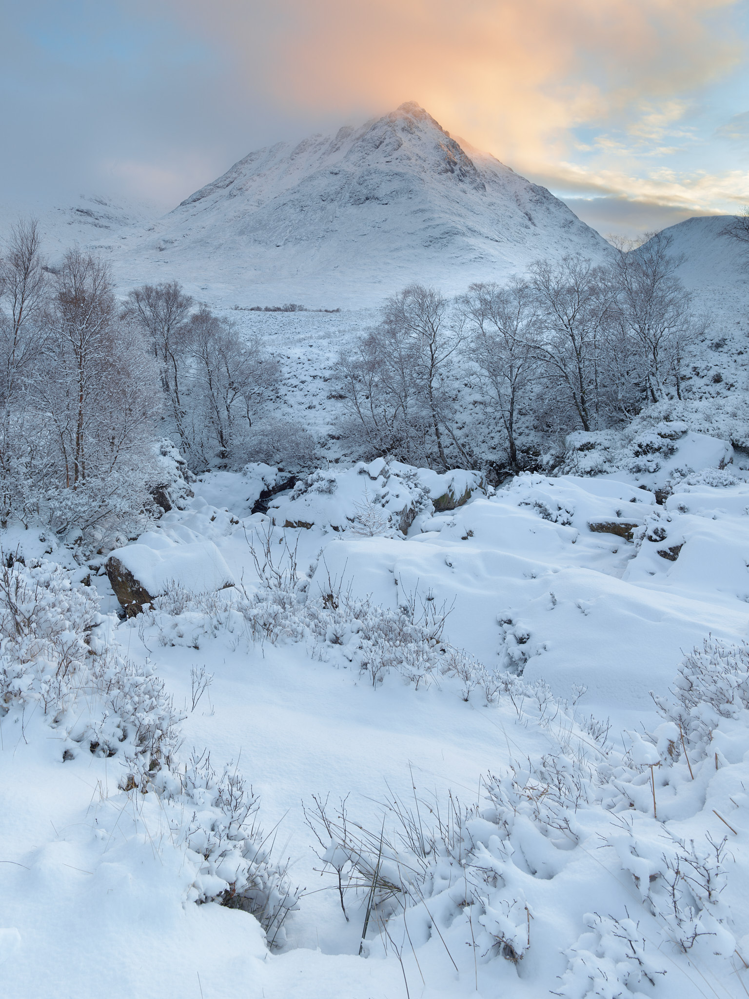
This scene was shot on an IQ3 so I used my handheld meter to spot the brightest point in the sky and added about two stops. If I recall I also had a two-stop graduated filter on the sky so I added on two stops for that. I do know I checked the histogram and the playback on the camera back afterwards to make sure no highlights were clipped. On my IQ4 I would again place the brightest highlights at the right-hand side of the histogram and check once it was taken that no highlights were clipped. On transparency film I would meter the scene like the IQ3 – and would have to live with the blocked out shadow details which digital preserved. On negative film I would spot meter the black shadows and place them on -1.5 to -2 trusting negative film to hold the highlights assuming a low-contrast development approach on black and white (N-1) followed by a scan or relying on the highlight latitude of colour negative film.
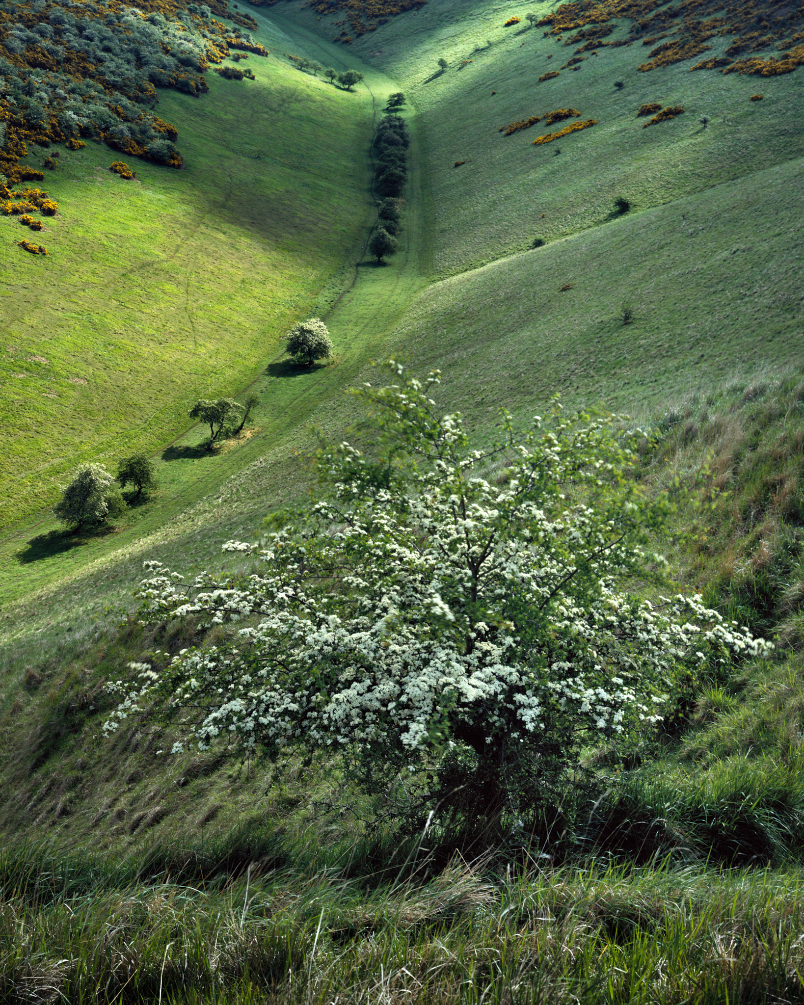
With example III shot on transparency film I metered on the sunlit grass and placed that on +1. On digital I would again place the highlights to the right-hand side of the histogram when the sun was out but leave plenty of space to avoid the risk of clipping. I would probably meter negative film like the transparency putting the sunlit grass on +1 given the lack of significant shadows. I had to pre-meter – in other words meter off some sunlit grass in anticipation of the scene lighting as there would be no time to meter then shoot for such a time-critical exposure.
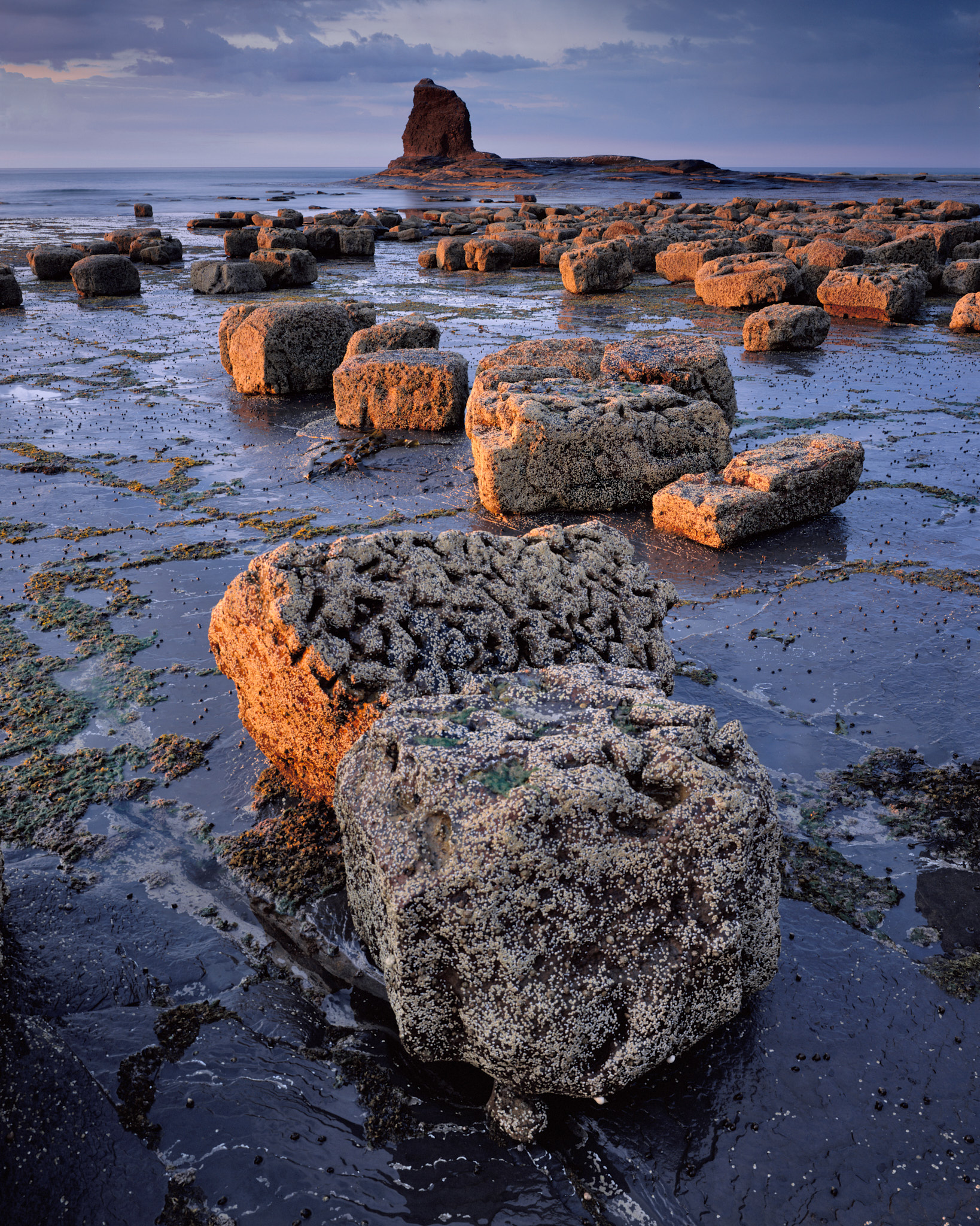
Example IV was again shot on transparency film with a two-stop graduated filter over the sky. So the bright spots in the sky were placed at +3.7 and the midtones checked to see where they would fall. On digital I would be checking the sunlit rocks to make sure they had not blown out.
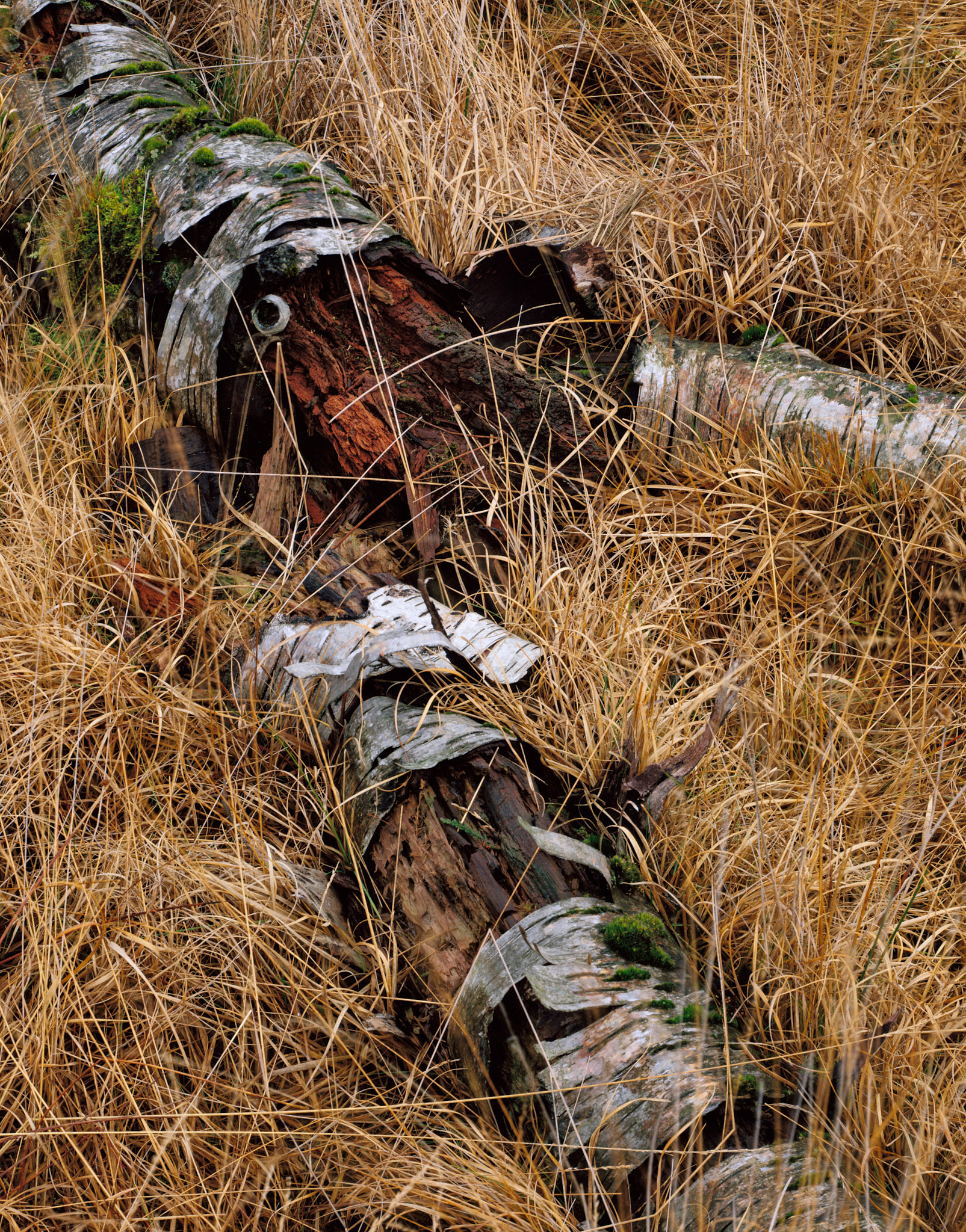
Example V was simple to meter on transparency film. I placed the yellow grasses on +0.5 and checked that the white birch bark was < +1.7 for that exposure. On digital I would expect a simple upside-down cup-shaped histogram which I would place the top of around the middle of the histogram – the key thing being again to check that the highlights for the birch bark don’t blow.
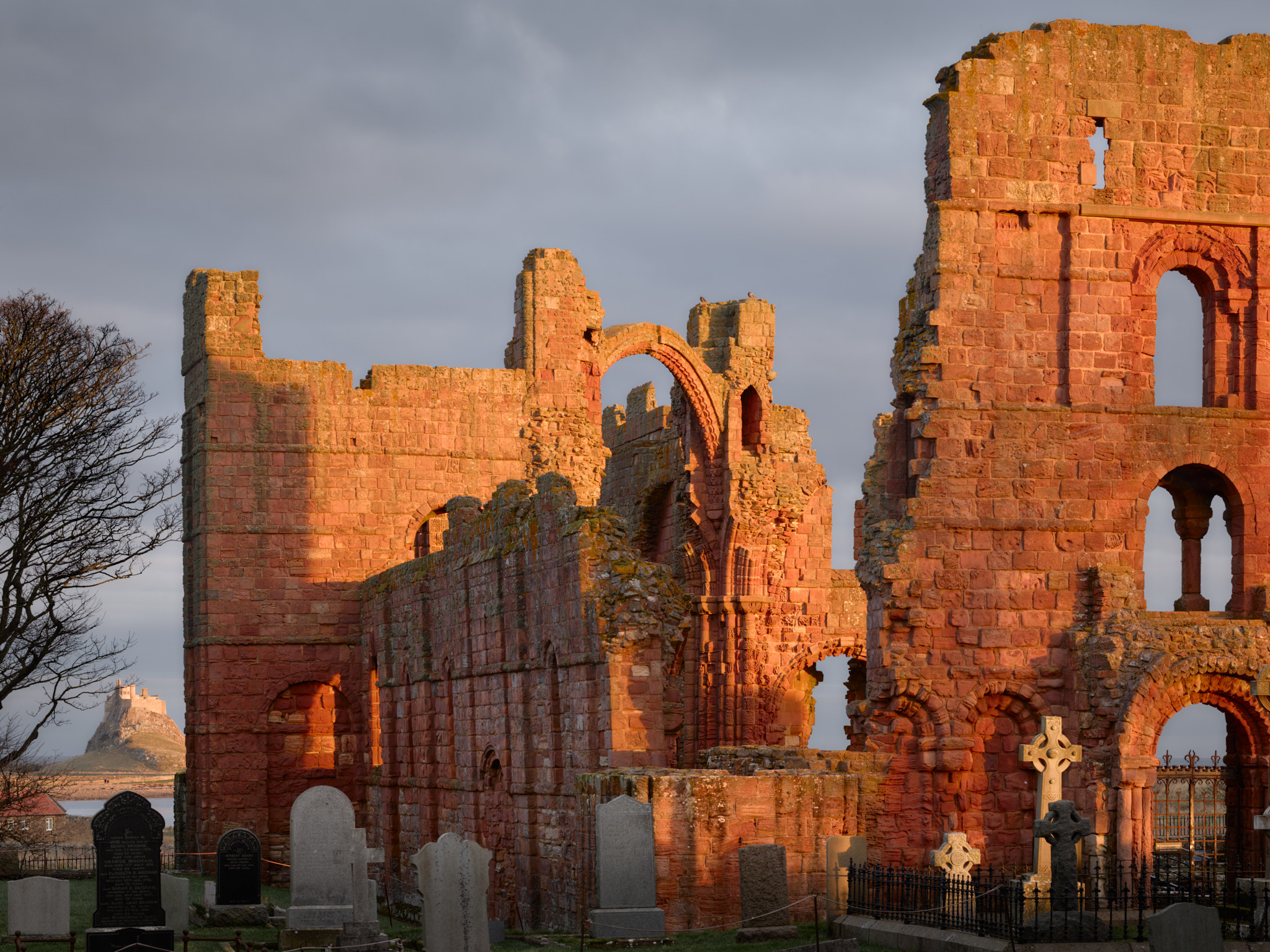
The pattern should be clear by now. Shot on an IQ4, I simply aimed to place the highlights at the right-hand side of the histogram close to the edge and checked the highlights after I shot. I had live-view switched on and was ready for the big spike in brightness that was to come when the sun got up – it would be easy to forget. There were no concerns about shadow detail.
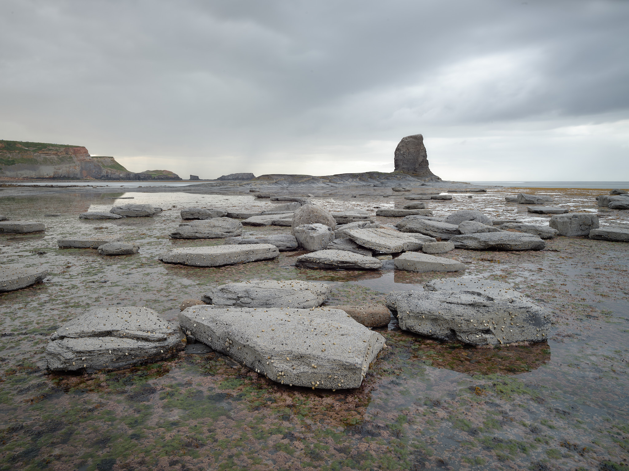
For Example VII I used a 2-stop graduated filter for the sky to help balance the image and was able to correct its impact on the scene in post – removing the over-darkening of the rock formation and cliff. I would have done the same with transparency film and on negative film metered from the base of the nab and probably put it on about -1 checking that the highlights come into the expected range of the film. In this situation I also used a long exposure – so ordinarily I would have added something like a 6-stop ND filter but in this case I used the Frame Averaging capabilities of the IQ4 150 to achieve a 10-second exposure.
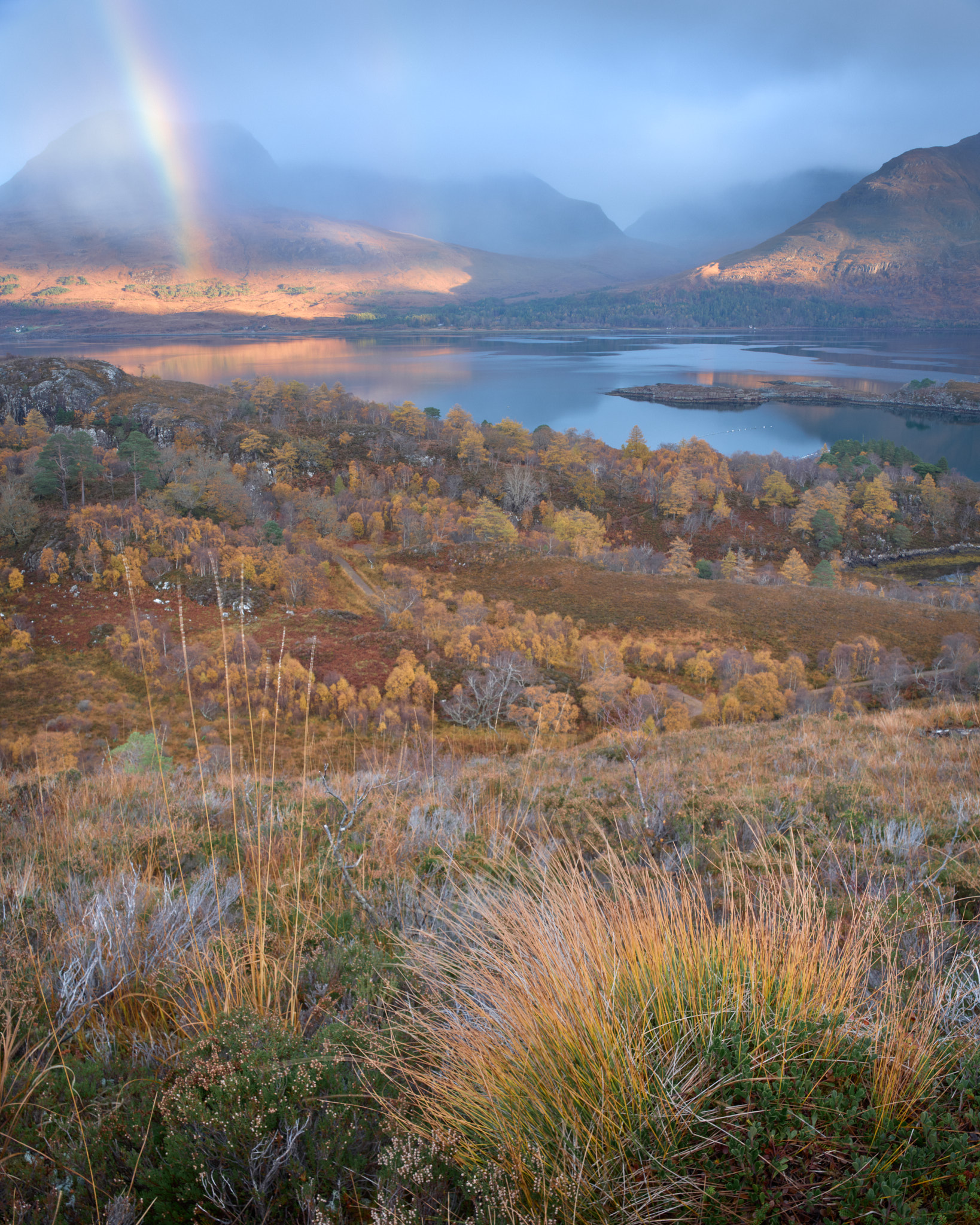
This dawn image had a large contrast range. If I recall I used three filters. A polariser to help emphasise the rainbow, a two-stop hard and a two-stop soft graduated filter. On a GFX 100S I used the histogram to place the highlights close to the edge of the sensor clipping point and checked the exposure using the image preview in camera to make sure the sky highlights were not blown. I shot this scene at sunset several years before in the first few weeks of using digital sensors on technical cameras and then I blew some of the highlights making it very difficult to process. In those days the GFX 50S (pre-BSI) would have poor-quality colour rendition from heavily recovered shadows. This time I was not going to make the same mistake!
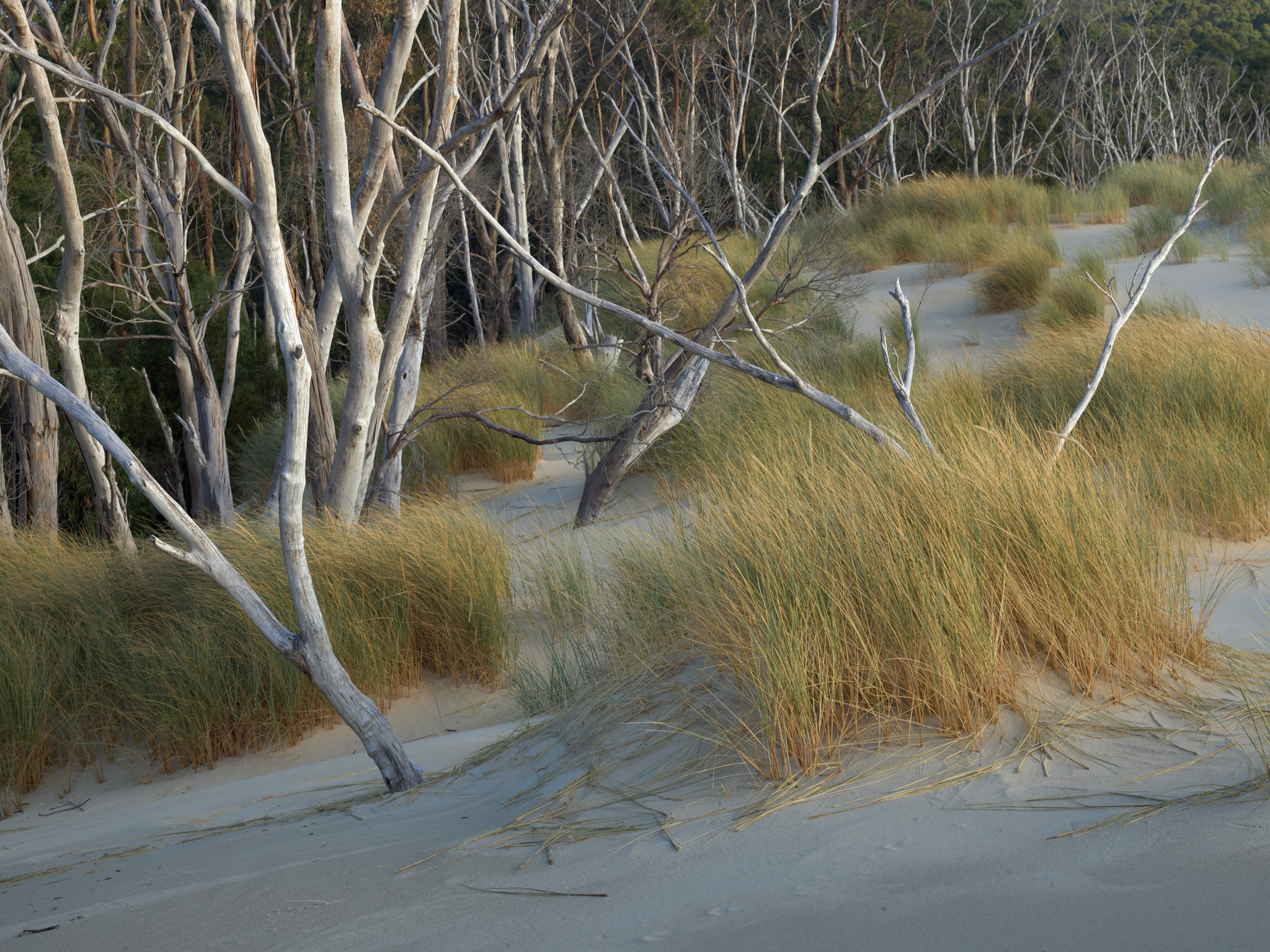
Although the live-view histogram tool makes metering a scene so much easier than it used to be on film, it still pays to look at a scene and ask yourself what are the important highlights. It means you can check these in camera. In this case the sunlit white tree bark is the highest risk component of the image and that is what we should set out to protect. So I made sure that on my IQ4 there was no chance of clipped highlights there using the image review tooling of the Phase – rather than the typical clipping review tool it has a colour-coded rendition of the image that shows different zones – I typically make sure that there are no white zones (close to or higher than +3) and instead the highlights are flagged as red zones (~+2 stops) to be confident the exposure is good. On transparency film I would meter from that sunlit tree and place it at +1.5 or +1.7 again accepting that the shadows might block up. On negative film I would target the shadows in the woods and place them on -2.
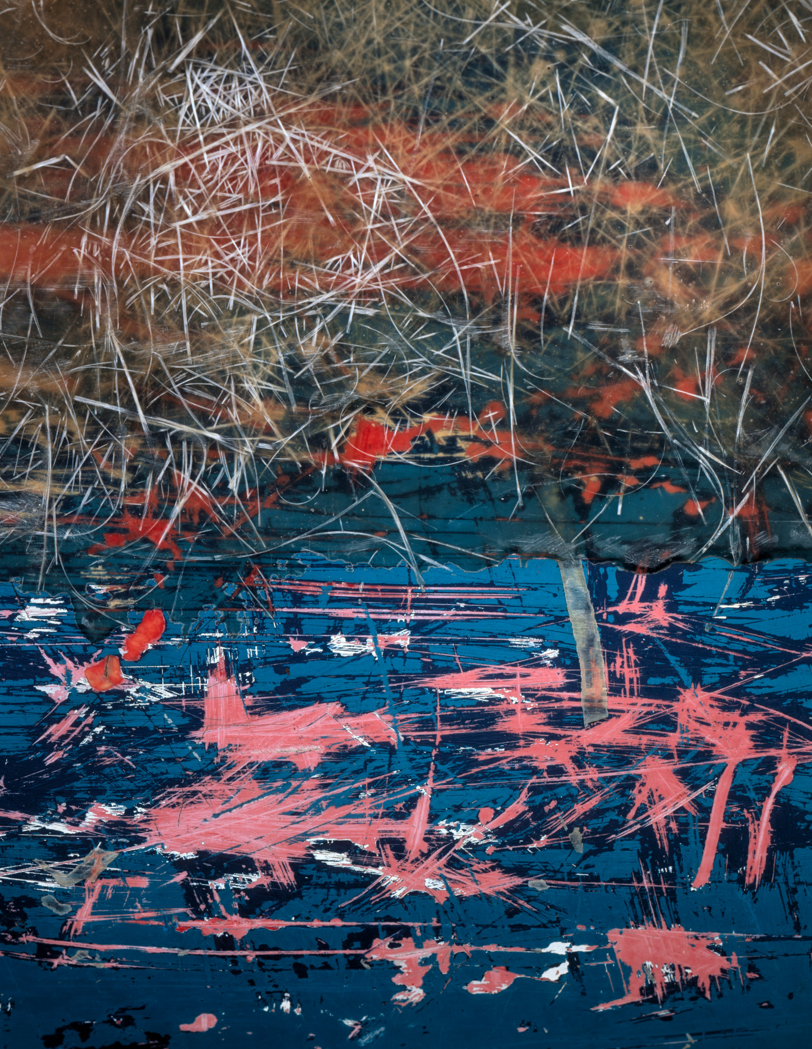
One huge advantage of the live-view histogram is the use with technical cameras for situations like this – where the image is around or just larger than lifesize. On transparency film this kind of image is a huge test of exposure craft. Made on Velvia film, firstly I had to find a target to meter – I probably spotted several points and took an average reading paying particular attention to the risk that the white spots would blow and that they are <1.7 stops from the selected exposure. My brilliant Minolta/Kenko light meter would allow that to be done. But then the hard work was not over. I would have to account for bellows factor – light fall-off from having such a macro setup. By this stage of my Mulgrave work I had created a table for each lens so that I could measure the rail extension with a tape measure and read off how many stops to add – in this case I expect it was around 1.8 stops. Today I would set up using my Cambo Actus and just make sure that the right-hand side of the live-view histogram is close to but not overlapping the clipping point. I would not like to go back to the days of having to do all the metering calculations in my head but it did keep one on one’s toes!